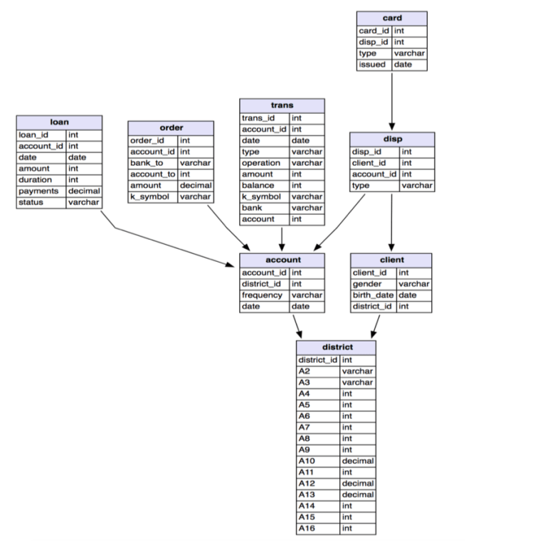
In today’s world, there is an increasing number of people who are looking to borrow money from banks. Unfortunately, there are also a lot of people who cannot afford to pay the money back. Loan default is one of the most critical factors that banks concern and that needs to be resolved. In order to reduce this problem, it is necessary to find out which type of people will likely default. I am going to use the bank dataset collected in 1999. It consists of 8 tables, which the status of the loan is described in the loan table.
Data Exploration:

To briefly discuss the loan status, the status column consists of 4 letters, which B as being default and A, C and D as not defaulting. According to the description of the label, A and C are stated as OK and no problem whether their contract finished or not. I also included D as not default, because the contract is not finished even though the client is in debt. However, it is clear to label B as default since they have not paid their loans despite the contract having to finish.

Data Preprocessing:
As mentioned in the data exploration section, I would like to aggregate the data based on loan_id, which is the account holders who borrowed money from the bank. So the purpose is to predict client’s behaviors about the loan for each account.
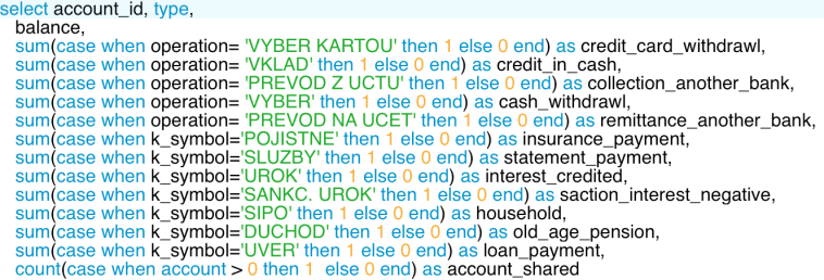
In order to use the categorical variables, I need to convert it to numerical values in order to apply the features on to the machine learning models. It can be done in Python as well, but I chose to do this on SQL in this project. After that, I left join all the tables there are on to loan_id in loan table.
As there are missing values in 6 different columns, we need to use Python to do some feature engineering to resolve this. In this case, I have used fillna() function to fill in the null values to zero and median values according to its characteristics.
Model Selection:
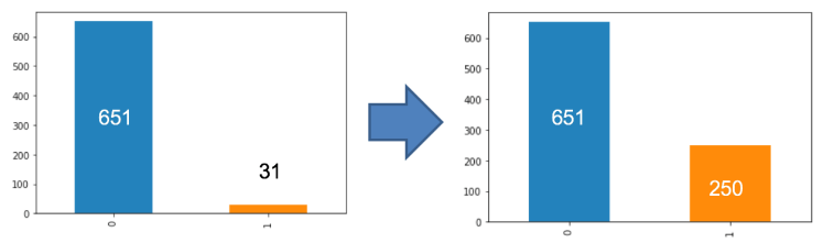
After joining the table, we can determine the number of clients who have gone default. As you can see on the bar graph, there is a significant difference in terms of how many clients who have gone default and who did not. In this case, the overall accuracy score can have high numbers, but it will have a lower f1 score. It is crucial for us to consider the f1score if we are dealing with cases like default, churns, and fraud detection cases. The f1 score determines both precision and recall, which means it will consider all the cases where we have thought the client went default but did not and the client’s that we have missed to label as default that actually did. One of the ways to resolve this problem is oversampling the minority class so that the result is not biased.
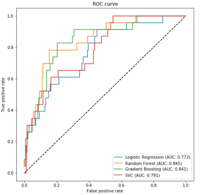
The machine learning algorithms I have used for these are Logistic Regression, SVC, Gradient Boosting, and Random Forest. I plotted these models for the ROC curve to calculate the AUC score. The best AUC score from the four models is Random Forest. Not only does Random Forest has the highest AUC score, it has an advantage of depicting important features.
Feature Selection:

 Top 5 features according to the graphs are loan_payment, maximum_trans_balance, issuance_after_transaction, and loan_amount. As you can see in the bar graph, the maximum transaction balance is higher and the minimum transaction balance is lower for the clients who are defaulted.
Conclusion:
In this project, I have experienced with handling an imbalanced dataset, which I have applied the oversampling technique to reduce the bias. After that, I found out that the most suited algorithm is Random Forest, which I have the highest accuracy as well as the f1 score. It is crucial for the banks to detect the default behaviours in the early stages and consider all the situations where it may cause the possible losses for the bank. I hope to dig deeper into this project by applying more algorithms and looking into more features.

Leave a comment